
Distributed training
To train on several devices, you give Trainer two objects. A MeshSpec says how many devices each of six named mesh axes gets, and MeshSpec.build arranges the devices into a jax.sharding.Mesh with those axes. A Layout maps the logical axis names that Dew’s modules give their parameters, such as embed and mlp, to mesh axes. Trainer uses both to initialize, place and update the training state, and XLA compiles the collectives that placement needs. The model, the objective and the data stay the same whatever mesh you choose.
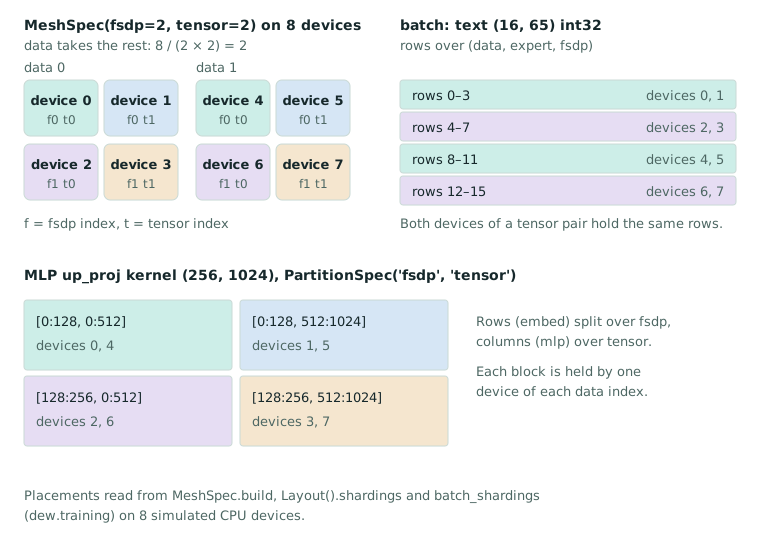
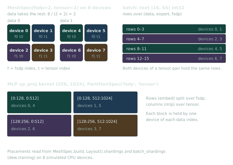
docs/assets/figures.py draws the figure from the placements that MeshSpec.build, Layout().shardings and batch_shardings return.
Example
Section titled “Example”This trains a small decoder on eight simulated CPU devices. --xla_force_host_platform_device_count must be set before JAX is imported.
import osos.environ["XLA_FLAGS"] = "--xla_force_host_platform_device_count=8"
import itertools
import jaximport numpy as np
from dew import Trainerfrom dew.data.dataset import Loaderfrom dew.optim import OptimConfigfrom dew.nn.backbones import CausalTransformerfrom dew.objectives.lm import LMObjectivefrom dew.training import MeshSpec
model = CausalTransformer(vocab_size=512, emb_features=256, num_layers=2,                          num_heads=4, mlp_features=1024, max_seq_len=64)rows = np.random.default_rng(0).integers(0, 512, (16, 65), dtype=np.int32)data = Loader(train=lambda partition: itertools.repeat({"text": rows}), val=None,               records=16, batch=16)trainer = Trainer(LMObjective(model, seq_len=64), OptimConfig(learning_rate=1e-3), key=jax.random.key(0),                  mesh=MeshSpec(fsdp=2, tensor=2))state = trainer.fit(data, steps=4, log_every=2)
kernel = state.variables["params"]["layers_0"]["mlp"]["up_proj"]["kernel"]print(kernel.shape, kernel.sharding.spec)print(kernel.addressable_shards[0].data.shape)
Training CausalTransformer from step 0 to 4: 2.2M parameters, on 8 × cpu, mesh data 2 × fsdp 2 × tensor 2, batch 16, float32step 2/4 loss 4.741 ce 4.741 perplexity 114.5 token_accuracy 18.8% step_time_ms 302.9 samples_per_sec 52.82 accepted 100.0% 0:00:01 leftstep 4/4 loss 2.140 ce 2.140 perplexity 8.499 token_accuracy 92.5% step_time_ms 154.2 samples_per_sec 103.8 accepted 100.0%Trained 4 steps in 0:00:02: first step after 1.32 s, then 5.9 step/s27.7% of the wall time in steps, final loss 2.140(256, 1024) P('fsdp', 'tensor')(128, 512)Each device holds a (128, 512) block of the (256, 1024) kernel, because the rows are split over the two fsdp devices and the columns over the two tensor devices. The kernel’s Adam moments are placed the same way.
Each MeshSpec field sets how many devices one axis gets, and the data axis gets the rest. The product of the fields must divide the device count, or MeshSpec.build raises LayoutRefused.
| Axis | MeshSpec field | Splits |
|---|---|---|
diloco | diloco | DiLoCo’s replica groups (Trainer(diloco=DiLoCo(every))): each group trains its own copy of the model on its own batch rows, and the groups average every every updates |
data | (the remainder) | Batch rows; parameters are replicated over it |
expert | expert | The expert dimension of mixture-of-experts layers, and batch rows |
fsdp | fsdp | Parameter dimensions the layout assigns to it, and batch rows |
tensor | tensor | The MLP hidden width, attention heads and vocabulary (Megatron’s split) |
sequence | sequence | Token positions, for sequence-parallel attention, and with fsdp the parameter dimensions the layout assigns to fsdp |
stage | stage | A stack of like layers (a decoder’s, a DiT’s or a ViT’s blocks, a UNet level’s transformers), into pipeline stages |
from dew.training import MeshSpec
print(dict(MeshSpec(fsdp=4).build().shape))print(dict(MeshSpec(fsdp=2, expert=4).build().shape))print(dict(MeshSpec(fsdp=4, sequence=2).build().shape))
{'diloco': 1, 'data': 2, 'expert': 1, 'fsdp': 4, 'tensor': 1, 'sequence': 1, 'stage': 1}{'diloco': 1, 'data': 1, 'expert': 4, 'fsdp': 2, 'tensor': 1, 'sequence': 1, 'stage': 1}{'diloco': 1, 'data': 1, 'expert': 1, 'fsdp': 4, 'tensor': 1, 'sequence': 2, 'stage': 1}MeshSpec also has replicas (host groups the data axis spans; see Multiple hosts).
A native mesh
Section titled “A native mesh”Trainer(mesh=...), Checkpoints.variables(mesh=...), dew.pipeline(..., mesh=...) and Pretrained.load(..., mesh=...) also take a jax.sharding.Mesh you build yourself, with axes of any names. Layout.rules maps the model’s logical axes onto them, and Layout(data_axes=...) names the axes a batch’s rows split over, which the run’s data shares, its batch placement and its row counts read (dew.mesh.batch_axes under the layout’s rules, which the trainer puts in context). A rule that names an axis the mesh lacks is refused by name, except Dew’s own role axes, which a mesh without them treats as size 1. The data and stage axes never hold a parameter. The expert exchange, sequence-parallel attention, the pipeline and the tensor-parallel heuristics run on the axes named expert, sequence, stage and tensor; any other axis, a second fsdp level or a context axis, holds parameters and rows as your rules place them.
from dew.training import Layout
from jax.sharding import AxisType
mesh = jax.make_mesh((2, 2, 2), ("replica", "zero", "zero2"), axis_types=(AxisType.Auto,) * 3)layout = Layout(rules={"embed": ("zero", "zero2"), "mlp": "zero", "vocab": "zero"},                data_axes=("replica", "zero", "zero2"))trainer = Trainer(LMObjective(model, seq_len=64), OptimConfig(learning_rate=1e-3), key=0,                  mesh=mesh, layout=layout)trainer.fit(data, steps=2, log_every=2)
jax.make_mesh makes Explicit axes unless axis_types says otherwise. The partitioner places Dew’s parameters, so their axes are Auto, and a rule that puts a parameter on an Explicit axis is refused by name; an Explicit axis can split the batch’s rows, which then sit where their type places them. A batch placed outside the trainer, by dew.distributed.batches.shard_batch say, reads the rules in context: put it under flax.linen.logical_axis_rules(layout.axis_rules).
Parameter placement
Section titled “Parameter placement”Modules declare logical axes such as embed, mlp, heads, kv, vocab and exp. Layout.rules maps each name to mesh axes in precedence order, and the default table, dew.mesh.DEFAULT_RULES, puts large dense dimensions on fsdp and expert dimensions on expert. Under MeshSpec(tensor=N), the widths that Megatron splits are also split over the tensor axis: the MLP hidden width, the query and key-value heads, the attention width that o_proj reads, and the vocabulary. The residual width is not split over tensor. When a rule’s mesh axes do not divide a dimension, Dew tries the next rule for that name, and if none fits, the dimension stays whole.
Layout field | Default | Meaning |
|---|---|---|
rules | DEFAULT_RULES | Logical axis name to mesh axes, in precedence order |
min_shard | 2 ** 16 | Parameters with fewer elements stay replicated |
tolerance | 0.02 | The fraction of shardable parameter elements that may stay replicated before Layout.check raises |
host | () | Train-state fields kept in pinned host memory between steps: "opt_state", "ema", or "variables" for a CPU-owned step |
host_parameters | () | Globs of variables an inference placement keeps in pinned host memory |
frozen_whole | False | Keep the frozen collection (a LoRA run’s base) whole over fsdp, split only over the other axes its rules give it |
To change one name’s placement and keep every other, drop the default table’s rules for that name and put yours ahead of the rest. This keeps the vocabulary off the tensor axis, whether fsdp can split it or not:
from dew.mesh import DEFAULT_RULESfrom dew.training import Layout
layout = Layout(rules=(("vocab", "fsdp"), *(rule for rule in DEFAULT_RULES if rule[0] != "vocab")))
A rule put ahead of the defaults without dropping theirs is only a preference: where it cannot place the dimension (its axis has size 1, or does not divide it), the default rules for the name behind it still apply. A rules mapping, or a sequence without the defaults, replaces the table whole. The defaults name some logical axes more than once as fallbacks, and a mapping keeps one rule per name, so build a variant from them as above and not as dict(DEFAULT_RULES).
A parameter that no module declares logical axes for is split on its largest dimension that the fsdp size divides. Layout.check raises LayoutRefused when more than tolerance of the shardable elements stay replicated, and it lists the largest replicated parameters. Raising tolerance only hides the problem, so fix the placement. A rule that puts a parameter on data or stage is refused.
The sequence axis’s devices compute their own positions with the same weights, as fsdp’s compute their own rows, so the two hold the training state between them. Whatever the rules put on fsdp is split over fsdp and sequence together wherever their product divides that dimension and the pair leaves the other axes’ splits as they are, and over fsdp alone otherwise. On MeshSpec(fsdp=2, sequence=2) a parameter the pair splits lies on each device as on MeshSpec(fsdp=4), a quarter of it, and so do its optimizer moments, its EMA copy and its gradient; on MeshSpec(sequence=N) an N-th. Parameters below min_shard stay replicated, and frozen_whole keeps the frozen collection whole over both. A step reads such a weight as it reads an fsdp split. torchtitan’s FSDP shards over its dp_shard and cp axes together in the same way. Layout.check counts the axes the rules name, so a sequence size that divides none of a parameter’s dimensions leaves that parameter whole over sequence without a refusal.
frozen_whole is for a frozen base that fits on each device. A frozen leaf has no gradient and no optimizer state, so splitting it over fsdp and sequence saves only its memory while the step gathers it whole forward and again backward. With frozen_whole=True each device keeps it whole over both instead (a tensor split stays), Layout.check counts none of its leaves, and a leaf host_parameters also names is kept whole in pinned host memory.
Optimizer moments and EMA copies have the same shapes as their parameters and are placed the same way. When a checkpoint is restored, Dew builds the restore template for the layout you asked for, so a run can resume on a different mesh as long as the parameter names and shapes match the saved state.
Activation placement
Section titled “Activation placement”The same table places activations. Its activation_ names put a batch’s rows on the data, expert and fsdp axes and its positions on sequence, and they put an activation’s heads, MLP hidden width and vocabulary on tensor. The model pins the residual stream, the attention heads and the MLP hidden width to these names with dew.nn.sharding.constrain, and the trainer compiles its step under flax.linen.logical_axis_rules(layout.rules). So when you change a rule, the activations move with the parameters.
Without those pins, GSPMD chooses each activation’s placement from the weights around it. On an fsdp mesh it split the residual width and all-reduced the partial products of every projection, and on a tensor mesh it gathered every weight, as fsdp does. A batch’s rows are never split over tensor. As in Megatron, every tensor shard reads the same rows and computes its own part of the width for them. When a rule’s mesh axes do not divide an activation’s dimension, the next rule for that name applies, or the dimension stays whole, the same as for parameters.
Some per-token work does not split any width that the tensor axis splits. Multi-head latent attention’s down-projections into its query and key-value latents, and DeepSeek-V4’s query latent and shared key head, read the whole residual, so under a tensor axis every tensor shard computed them over every token. At DeepSeek-V3’s shape under tensor=8, that made a step cost 1.133 times one device’s matmul FLOPs.
So where the tensor axis’s link is fast enough, these projections run on each tensor shard’s own tokens. Their input is placed as SPREAD, whose activation_spread rule splits positions over the tensor axis as well as the sequence axis, and the latents are gathered back for the up-projections, which are split by head. That saves (T - 1)/T of the projections’ FLOPs. It adds gathers of the latents and of the residual’s gradient, plus a sum of the projections’ weight gradient over the tensor axis.
dew.nn.sharding.down_projection decides for each projection while the step is traced. It spreads when the link can move those extra bytes in no more time than the device, running at its peak rate, would take for the FLOPs saved. The peak rate is the fastest the device can run those FLOPs, so at any real utilisation they take at least that long, and spreading cannot slow the step. The trainer measures the link once per mesh with an all-gather over the tensor axis (dew.training.distributed.link_bandwidth). Every process uses the lowest figure in the pool, so they all compile the same program. For each axis it measured, StepCompiled records that figure and whether a projection spread.
At DeepSeek-V3’s widths in bf16, with 16384 tokens per microbatch, an RTX 3090 needs 20.3 GB/s. On 4x RTX 3090 (PCIe 3.0, one host), the all-gather over the NVLink pair moved 31.0 GB/s, so that pair spreads; the PCIe pair moved 5.8 GB/s, so it does not. An H100 SXM needs 283 GB/s, under NVLink 4’s nominal 450 GB/s per direction. No spread step has been timed on NVLink or on a TPU. Nothing is measured on a device that the peak table in dew.telemetry.instrumentation does not name, a CPU among them, so there the projections stay on every token. To decide for such devices, or as another machine would, state the link: Trainer(..., links={"tensor": Link(bytes_per_second, flops_per_second)}), with Link from dew.nn.sharding, or on a run --set trainer.links='{"tensor": {"bytes_per_second": 4.5e11, "flops_per_second": 9.9e14}}', and the same rule weighs it. To keep these projections on every token whatever the link, map activation_spread to the sequence axis alone in your rules.
The sequence axis has the same problem with a cross-attention’s context, such as SD’s 77 text tokens. The sequence axis does not divide a length like that, so every sequence shard projects the whole context into keys and values. On a CPU mesh under sequence=4, before the split below, that made the conditional UNet’s step cost 1.57 times one device’s FLOPs. dew.nn.sharding.split_positions decides by the same rule, using the sequence axis’s measured link. Where splitting pays, each shard projects its share of the positions, padded with zero rows to a multiple of the shard count.
The split adds a sum of the projections’ weight gradients, which is a lot of bytes next to the FLOPs it saves, so a GPU’s link rarely pays for it. At SDXL’s widths, with 8 rows per sequence group and no head sharding, an H100 would need 2.47 TB/s once the extra work on padded positions is subtracted from the savings. So in that configuration every sequence shard projects the whole context, which costs FLOPs but no collectives. The link calculation uses the output head width that the active layout rules leave on each device.
The cross entropy scores each device’s own tokens. It runs in a shard_map over the axes that hold the tokens, plus any other axis whose size divides the token count, and every device holds the whole head. Only the head’s gradient and the loss’s sums cross devices.
Host memory
Section titled “Host memory”Layout(host=("opt_state", "ema")) keeps the optimizer state and the EMA copy in pinned host memory between steps. Once the step’s gradient is ready, it brings them to the device a chunk at a time. A chunk holds the leaves the update reads together: under AdamW, one parameter’s two moments and its average. Each chunk goes back to host memory as soon as it is updated, so the device holds about two chunks of the state instead of all of it. The update is the same one, so the values match a device-only layout. Some commits read the whole state at once and bring it whole: an update that reads every leaf together, a window of several microbatches (which commits under a conditional), and a dynamically scaled loss (which accepts the commit only if the whole updated state is finite). The memory planner counts what the commit stages either way. Checkpoints save and restore this placement. The transfers add time to every step, so measure the step time with and without them.
When a checkpoint of host-resident state is saved, training waits until it is written. Orbax copies a device array to host memory before its asynchronous write, but it writes an array that is already in pinned host memory straight from the array’s own buffer. The next step donates that buffer, and a GPU refuses the donation while the write is still reading it. So the step after a save waits for the write, and no extra memory is used.
Handing Orbax a copy would make the step wait only for the copy. But the copy would stay in pinned host memory until the write finished, and for fp32 Adam moments and EMA it is 12 bytes per parameter, or 84 GB at 7B parameters, on a host that keeps the state there because it has no room elsewhere. On an RTX 4080 host with a consumer NVMe drive (657 MB/s direct writes), writing a 6 GiB host-resident state took 18.4 s, where the copy would have taken 3.6 s and 8.4 GiB more peak memory. At 7B parameters that is about 4 minutes per checkpoint on that drive, against 20 to 50 s for the copy, and proportionally less on a faster drive. Choose checkpoint_every with that in mind. On that host, Orbax’s write path itself held about 0.9 bytes of transient memory per byte written, whether or not it was given a copy.
Layout(host=("variables",)) moves the whole train state to the CPU, the optimizer state, the EMA and gradient accumulation included. The optimizer update runs on a CPU companion of the mesh, and the parameter copies on the accelerators are read-only snapshots for the step. Each process needs at least as many CPU devices as it has accelerator devices, set before JAX initializes (JAX_NUM_CPU_DEVICES, or --xla_force_host_platform_device_count in the XLA flags). Its CPUs beyond that, and processes the mesh leaves out, stay out of the companion, and a process with fewer is refused before any model state is allocated. Neither the layout nor the trainer changes the count.
Layout(host_parameters=("params/layers_*",)) keeps a root decoder stack in pinned host memory for inference. Each model declares every physical stack with a DecoderBank, which records the stack’s layer namespace (the same below every variables collection) and its StackView. MultimodalTransformer puts its decoder under language_model, and DiffusionGemma declares text once for the scope its encoder and decoder share. To select a nested stack, use a path such as params/language_model/layers_* or params/text/layers_*.
A scanned decoder declares one bank per run of like layers, and an unscanned decoder declares one bank per layer. Both stream through the same fetch loop, which holds the current layer and the next one. A LayerBanks source’s place(model, layout=...) reads each physical bank once and rejects two different views of the same namespace. Selected leaves keep their FSDP and tensor PartitionSpecs, and external cache arrays stay on the device under their logical per-layer paths. GPU peak-memory bounds, and whether the transfers overlap with compute, have not been measured. Trainer.place rejects host-parameter layouts, because Dew has no backward pass or optimizer path for them.
On a TPU, pinned banks keep their layer axis major-most in physical memory. A fetch keeps that axis until the copy reaches device memory and squeezes it out there, which avoids incompatible host tile bitcasts and still transfers one layer at a time. Bank sources must honor any JAX Format given in their placement; both built-in sources do.
dew.inference.LayerBanks has two adapters for real use:
CheckpointBanksreads Dew run checkpoints bank by bank.HeldBanksborrows an existing variables tree without donating or deleting it. The whole source stays in memory while the destination banks fill up, so it can hold two copies of the model at once.
Both read the entry leaves, the ones outside the declared stacks, and both accept namespaces relative to a collection for bank reads. Media, embeddings and heads stay entries even when they share a parent module with a decoder. Each entry or bank is placed before the next read starts. CausalTransformer(bank_layers=N) limits how large a bank is when it is built; it does not cap the pinned allocator or free the source’s own storage. StackView still exposes the logical layers_N paths for saving and export. Synthetic generation is only in tools/benchmark_host_offload.py.
Loading a published checkpoint onto a mesh streams it leaf by leaf, though it does not stream banks into pinned host memory. Pretrained.load(source, mesh=MeshSpec(...), layout=Layout(...)), which dew.pipeline(source) calls, never builds the translated model on the host. Each decoder leaf is a recipe over the memory-mapped checkpoint that says which stored tensors to read, whether to transpose them or stack experts, and the storage dtype. jax.make_array_from_callback then reads only the part each device holds, and casts and transposes that part alone. The mapped pages are released once the leaf is placed. So the host holds at most one device shard of one leaf at a time, plus the towers, projectors and any dequantized quantized tensors, which are still built whole.
On one RTX 4080, loading Qwen3-0.6B in float32 this way peaks at 3.9 GB RSS, against 6.2 GB for loading first and placing afterwards. On an 8-device CPU mesh the figures are 4.0 GB and 5.9 GB, and 2.4 GB of that is the placed model itself. For Qwen3.8-27B (55.6 GB in bf16) on an 8-device mesh, the recipes cover 54.6 GB of the checkpoint, the largest single read is 0.32 GB, each device holds 6.95 GB, and the vision tower built on the host is 0.92 GB.
Host-parameter placement works only for decoder stack variables. Dew rejects a selection that includes an embedding table, a head or a prediction depth. Matching leaves of every layer in a bank must have the same memory kind and PartitionSpec. The stage pipeline and training through a banked store are rejected. In JAX 0.11.1, reverse-mode autodiff through the fetch loop does not lower, because its transpose asks for a dynamic_update_slice whose operands are in different memory spaces. A small forward-mode probe agrees with resident placement, but that probe does not show that backward re-fetch or training works.
Every host-resident weight you select is copied to the device on each forward pass, including every decode step, so PCIe transfers can take most of the time per token. tools/benchmark_host_offload.py reports local addressable-shard bytes, the device and host compiled-memory fields, process RSS and execution times. Its bytes per token divided by the decode latency is an end-to-end effective rate, not a measurement of PCIe bandwidth alone.
An earlier synthetic BF16 bank load of 18.00 GiB (144 layers, width 2048, bank_layers=8) reported 18.74 GiB final RSS and 37.9 GiB peak RSS. The saved load probe synchronized every bank, so a backlog of asynchronous work alone cannot explain that peak. The numbers do not separate temporary storage, allocator reservation and duplicate driver mappings. There is no completed result yet for generating on a GPU with a model larger than device memory, and no throughput result. Looking further into the allocator needs a small process tree with a hard memory cap, swap accounting and RSS/PSS measurements. The earlier oversized runs with an RSS watchdog are not a safe way to do it.
GPU memory outside XLA’s pool
Section titled “GPU memory outside XLA’s pool”XLA preallocates a share of each GPU’s memory as its pool. A step’s collectives also allocate NCCL communicators, and those buffers live outside the pool: NCCL takes no allocator from its caller. cuBLAS’s workspaces and the loaded kernels sit outside the pool as well. XLA keys a communicator by its devices and its kind, so a step whose collectives use another device grouping, or a collective-permute beside an all-gather, makes another communicator over the same GPUs.
import dew sets NCCL_RUNTIME_CONNECT=0 unless you set it yourself. NCCL then connects a communicator’s rings, trees and NVLS peers, and allocates their buffers, as it creates the communicator, where XLA returns a failure to every rank as an error. Under NCCL’s own default since 2.22, those peers connect at a collective’s first launch. There, a GPU that fails to allocate leaves its peer waiting inside XLA’s first-call rendezvous, and XLA ends the process after 40 seconds. Connecting at creation allocates those buffers at once, even for a collective the program never runs, and it takes longer to create the communicator. Point-to-point connections, which an all-to-all and a collective-permute make, still connect when a peer is first sent to, whatever the setting, so Dew leaves room for them as well.
On a host of two or more GPUs, before the backend opens, prepare_process sizes the pool to leave the communicators their room at NCCL’s full speed:
- A child process (
python -m dew.communicators) measures each group size that divides the host’s GPUs. For each size it makes a collective’s communicator, connects an all-to-all to every peer, and connects a permute along each directed pair of GPUs in turn, in a communicator of its first GPUs and in one of each pair alone. NCCL picks each peer’s transport separately and can route a connection through a third GPU of the communicator, so each pair keeps its bytes on its two GPUs and the most on any other; a communicator is charged a pair’s bytes on its ends, and the most beside it on every other member, since NCCL may route the pair through any of them. It reports the bytes each step took on a GPU, and the bytes the runtime took beside its pool. - The answer is kept in Dew’s cache under
communicators/. It is keyed by the GPUs’ names and PCI places, the driver, NCCL’s version, everyNCCL_*setting, every XLA flag that sets NCCL’s communicators, and the JAX version. A host pays for the measurement once per configuration. - The pool’s upper bound is the share your run names, read in one place (
dew.devices.pool_bound): yourXLA_PYTHON_CLIENT_MEM_FRACTION; Dew’s 95% if you name nothing; or JAX’s 75% if you name preallocation or the allocator without a fraction. The pool shrinks below that bound only as far as it must to leave room for a collective’s communicator, an all-to-all’s peers and a permute’s peers over every GPU, plus the runtime’s. No NCCL channel or buffer is cut to fit. The pool only has to hold the compiled step, and the fit check holds the step to it as before. Dew logs the share it took once, and the fit check’s record carries it into the run record (pool). - Every program Dew compiles, steps and evaluations alike, passes one compile point. There, its communicators are read from its program: each device group of its collectives, each all-to-all’s group and each GPU’s permute peers. Those communicators stay made, so they are held together with those of the programs compiled before. A program that needs more than the room left is refused before it runs, with an error naming the bytes, instead of stalling in a collective.
None of this happens in five cases:
- a process that joins a pool of processes, whose communicators span hosts and so need network buffers a single host’s child does not make;
- a pool of no fixed share (
XLA_PYTHON_CLIENT_PREALLOCATE=false, orXLA_PYTHON_CLIENT_ALLOCATOR=platform); - a host of fewer than two GPUs;
- a process that asks JAX for no GPU;
- a process whose backend has already opened.
If a step that fit fails on its first run anyway, Dew raises the failure as the step’s (dew.training.memory.FirstRunFailed). The error includes each GPU’s free bytes outside the pool, labelled outside, both at the fit check and after the failure.
An example of the failure this prevents: a LoRA fine-tune of Qwen3.5-9B on two H100s with XLA_PYTHON_CLIENT_MEM_FRACTION=0.97 left 2,264 MiB free outside the pool on a GPU. Its step’s collectives used two communicators, each with 24 collective channels, 32 point-to-point channels per peer and 16 NVLS channels. One GPU entered the first all-to-all, and the other never did.
Rematerialization
Section titled “Rematerialization”CausalTransformer(remat=...) sets which activations of each decoder block the backward pass recomputes and which it keeps. The value is a policy. The default, None, recomputes nothing, and "full" keeps only the block inputs. The other names in dew.nn.backbones.decoder_block.REMAT_POLICIES are minimal, minimal_with_conv, minimal_with_scan_and_conv, minimal_with_context, save_dot_except_mlp, save_dot_with_context_except_mlp, save_dot_except_mlpwi, save_qkv_proj, save_out_proj, minimal_offloaded and qkv_proj_offloaded. Each keeps some of the named projection outputs (q_proj, k_proj, v_proj, kv_proj, context, scan, conv, o_proj, gate_proj, up_proj, down_proj) or offloads them to host memory: context is a mixer’s output, attention’s or a recurrence’s, and scan a recurrence’s alone, an SSM’s or a delta rule’s. They trade recompute time for memory the same way MaxText’s recipes of the same names do. You can also pass a record with your own lists, such as {"save": ["q_proj", "k_proj", "v_proj"], "offload": ["gate_proj", "up_proj"]}. Every policy trains the same model. tools/benchmark_decoder_remat.py --remat <name> reports the residual and compiler memory of one configuration.
Batches
Section titled “Batches”Dataset.batch is the global batch size. Dataset.train(partition) and Dataset.val(partition) read one share of every global batch, and DataPartition.of(mesh) returns this process’s DataPartition(index, count, readers, reader). Processes whose devices hold the same rows read the same share. For example, when a stage or sequence axis spans processes, several processes hold one row shard, and they count as readers of one share. A loader takes its records index::count, so global batch k holds the same records at every process count. shard_batch assembles the shares into global arrays of whole rows.
For custom data, read only the share that the partition you are given describes. Two readers of one share must read the same records in the same order, so a source that returns rows in whatever order its fetches finish, such as UrlStream, refuses a partition with more than one reader. If each process repeats the full dataset on its own, the run trains on a different distribution.
The placement helper treats rank-two and rank-three arrays as sequences, and it can split their second dimension when the sequence factor divides it. It keeps the non-batch dimensions of image and video tensors whole. Check custom rank-three data yourself, because the rank of an array does not tell the helper whether its second dimension really holds token positions.
Sequence parallelism
Section titled “Sequence parallelism”MeshSpec(sequence=N) splits the token positions of every sequence over N devices, and each attention call uses one of two exact exchanges.
The all-to-all follows DeepSpeed Ulysses. Each device trades its slice of the positions for a slice of the heads, attends over the whole sequence and trades back, so no device holds a whole key or value. It runs when tensor times sequence divides the number of query heads and sequence divides both the query and key lengths. Every other call gathers the whole keys and values next to split queries, which works for any head count and any key length.
Where both can run, a causal, windowed or masked call uses the all-to-all, because its kernel skips the masked blocks. The gather gives its kernel an explicit mask, which no kernel skips, and it took two to four times as long for causal attention. A call with no mask uses whichever exchange sends fewer bytes. On the gather path, a causal or masked call stripes query chunks to balance the work, so its sequence length must be a multiple of twice the number of sequence shards. Multiple hosts gives the measurements and the byte count.
A window that cuDNN accepts as its window flag runs through the all-to-all like any causal call, and the kernel skips the blocks outside the window. Local attention runs banded in the other cases: packed documents or sinks on cuDNN, a validity mask, a window on XLA, and chunks. A banded layer whose span fits in one shard’s slice needs no exchange. Each device attends its own positions, and one shift brings its first block the previous device’s last window keys and values, with their positions, segment IDs and validity. A layer with a wider span uses the all-to-all, like a dense call.
A token window has seq_len + 1 IDs, and the model reads seq_len positions. Check the model length as well as the shape of the batch array. Packed segments, windows and rotary positions must stay aligned.
Mamba-2 layers split the sequence the same way, so a hybrid of Mamba-2 and attention layers trains under MeshSpec(sequence=N). Each device convolves its own slice, reading the last conv_kernel - 1 tokens of the previous device’s slice, and runs its scan from a zero state. It then needs the state that the earlier slices leave. The devices pass each slice’s total decay and final state, [batch, heads, head_dim, state_size] in fp32, between them in ceil(log2 N) + 1 shifts (a parallel prefix scan), and each device adds that state’s decayed contribution to each of its outputs. Packed documents reset the state and the convolution at every segment change, including a change that falls on a slice boundary. A row with padding runs as it runs on one device: a padded slot neither reads nor advances the convolution or the state. Each real token’s convolution reads the conv_kernel - 1 real tokens before it in its document, wherever they lie, gathered from every earlier slice, so a pool of processes, which always carries validity, trains a hybrid sequence-parallel too. Decoding stays on a mesh with sequence=1. The sequence length must be a multiple of N, and each slice needs at least conv_kernel - 1 tokens. The tensor axis does not split the Mamba-2 scan, so every tensor shard runs the scan over the whole width.
Cached autoregressive generation needs sequence=1. A mesh that trains with sequence parallelism may still be unable to run the decode cache.
Layer scan and pipeline
Section titled “Layer scan and pipeline”scan_layers=True groups compatible consecutive decoder layers into a Flax scan, and the stored variables stay per layer. Scanning can cut compile time, but it adds stacking and loop overhead, and it does not promise a flat compile time or faster steps. Measure it at the model size and on the backend you plan to use.
Whatever scan_layers says, init draws each run of two or more like layers under one scan, so its program has one draw per run instead of one per layer. At a given seed those layers get new values from the same distribution, and the draw depends on bank_layers, which splits the runs. So a run recorded with a Dew version that initialized layer by layer starts from different weights at the same seed. Init under a stage mesh or with decode=True still runs the plain loop.
MeshSpec(stage=N) turns on the GPipe-style pipeline, and Trainer(microbatches=M) (--trainer.microbatches) sets how many microbatches a step feeds through its stages, one a stage by default. The layer pattern must repeat across stages and split evenly between them. A stack of like layers is pipelined: a decoder’s layer stack, a DiT’s blocks (a hybrid’s SSM and attention blocks where their pattern repeats every stage), a JEPA encoder’s or predictor’s blocks (a video’s spatial and temporal pairs), and each UNet level’s transformers (SDXL’s levels of two and ten). Embeddings, the output head, a UNet’s residual blocks and other operations outside the stacks are not split across stages; a stack the stages do not split evenly runs whole on every stage. TREAD’s routes take part of the tokens through a span of the blocks, which no pipeline stage’s one program runs, so a routed DiT trains on a mesh without a stage axis. The trainer refuses a stage axis on a model that runs no pipeline, such as FlaxDiff’s UNet, whose levels hold one transformer each, because every stage would compute the whole step. That refusal raises dew.mesh.LayoutRefused, a ValueError that names the axis and a layout that does run. Any other error on a layout is a defect.
Microbatch m takes rows m, m + M, m + 2M and so on, so each microbatch keeps its rows on the batch shards that already hold them. For that to work, M must divide the number of rows each device holds. For example, a batch of 8 rows over 4 row shards gives each device 2 rows. With four microbatches, some devices would have no rows in a given microbatch and would compute another microbatch’s rows again, so a stage × fsdp step would cost 1.43 times one device’s matmul FLOPs, where the pipeline bubble accounts for 1.25. The pipeline refuses that schedule. It names a microbatch count that divides the rows a device holds, and a batch size that fits the count you asked for. With 16 rows the same layout costs 1.20 times.
Each device stores only its own stage’s layers of each pipelined stack, with their optimizer state and EMA: about 1/N of the stack (Layout(stage_local=True), the default). Dew’s optimizers read a stacked leaf as its stored layers, so weight decay, Muon and its variants, LAMB, parameter groups and int8 moments act per layer. A checkpoint holds every layer as one device’s would and resumes on any stage count. fit returns and Observe reads the state as the run holds it, with no copy of every layer on every stage; the model reads it off the mesh as its stored layers, fit(state=...) takes it back, and Trainer.stored gives every layer whole for a reader by layer name (an export), at the memory replication takes. Three cases keep every layer whole on every stage, with the memory of replication: Layout(stage_local=False), an optax transformation Dew does not build that may read a parameter whole, and Gauss-Newton or DiLoCo. A run whose objective declares no pipelined stack logs that it keeps every layer whole. Some mixed layer patterns and KV-sharing configurations cannot use this pipeline. Cached decoding also needs stage=1.
Dew does not implement a 1F1B schedule.
Kernels and precision
Section titled “Kernels and precision”With "auto", a call that asks for arithmetic no fused kernel performs takes the reference path on every backend: a matmul precision above the default, a softmax outside fp32, or a compute dtype other than the inputs’. A bf16 call on a GPU older than sm80 takes the reference path too. Otherwise, on a GPU, attention uses cuDNN when the shape, dtype and requested features fit its supported path, and XLA for other calls. On a TPU it uses the Pallas splash kernel when the call qualifies, and XLA otherwise. A call qualifies with bf16 or fp32, query and key lengths that are multiples of 128 and at least 512, a mask that splash can describe, no additive bias, and whole sequences at the kernel. The sequence-parallel all-to-all gives the kernel whole sequences; the key/value gather does not. Packed masks and optional attention features can change which kernel runs and how much memory it uses.
Qwix quantization is an optional, experimental training path with int8 and fp8 matmuls. It keeps full-precision master parameters and changes the numerics. In the RTX 4080 measurements on Performance, fp8 did not make steps faster at the sizes tested.
On a GPU, XLA’s Triton GEMM fusion computes some int8 dots as two or four times their product, without an error (openxla/xla#51016). So every program Dew compiles over a model quantized to int8 compiles its GEMMs on cuBLAS instead. A program you jax.jit yourself over such a model takes the same options: jax.jit(f, compiler_options=dew.nn.kernels.options.compiler_options(model)). With CUDA 13, cuBLAS refuses some int8 shapes (on an A100, a contraction of 16 or 48), and a program with one fails to compile instead of computing a wrong result.
Several hosts
Section titled “Several hosts”The JAX process pool must be initialized before any device array or model is created; the built-in recipes do this first. Each host needs the same software, access to the data and a reachable coordinator. dew launch starts a pool over ssh or under Slurm, and MeshSpec(replicas=N) keeps fsdp inside a node while the data axis spans the nodes. Multiple hosts covers both and how to rehearse them on one machine, and Cloud TPUs covers TPU provisioning.
The local process-pool tests run real jax.distributed processes. They do not cover network failures, remote storage, TPU collectives or cluster preemption.
Checking a distributed run
Section titled “Checking a distributed run”Before booking the GPUs, read what the run would hold on them. On a CPU host, start Python with as many simulated devices as the run has GPUs, as this page’s first block does (XLA_FLAGS=--xla_force_host_platform_device_count=8, set before JAX starts). Build the trainer as the run will, and validate it with one global batch against the memory each GPU’s allocator will have, 95% of the GPU in a training process. Here the run is the model above on eight 80 GB H100s, pooling four steps into each update:
trainer = Trainer(LMObjective(model, seq_len=64), OptimConfig(learning_rate=1e-3), key=0, mesh=MeshSpec(fsdp=8), accumulation=4)report = trainer.validate({"text": rows}, steps=400, capacity=int(0.95 * 80e9))print(report.leaves["variables/params/layers_0/mlp/up_proj/kernel"])print(max(report.device_bytes.values()), "bytes on the fullest device")print(report.batch_axes, report.collectives, report.unbound)validate places nothing. It reports each leaf’s split and the part each device holds, the bytes each device keeps between steps (parameters, optimizer state, EMA and the gradient accumulator), the axes a batch’s rows split over, the collectives a step runs over each mesh axis (an all-gather and a reduce-scatter over fsdp, and over sequence where it holds the state in shares beside fsdp, an all-reduce over tensor and over the data axes), and the logical axes your rules leave unnamed, whose dimensions stay whole on every device (a parameter none of whose axes a rule names takes the shape heuristic). It raises LayoutRefused when that state alone is over a device’s capacity. On the GPUs themselves fit runs the same check against each GPU’s allocator limit before it places anything, and the plan’s fit check counts the accumulator and copies a step adds before it builds them; trainer.validation then holds the report of the plan the run takes. The step’s activations and other temporaries come on top; the plan checks them against the compiled step on the GPU. A CPU host builds no narrow copies, the bf16 copies a GPU step reads of fp32 parameters, so it leaves out their 2 bytes a parameter.
Compare a small global computation under each placement you plan to use: the loss and gradients, record identity, optimizer and EMA state, and a save and restore. Record the compiler and backend versions and the tolerances used. A device count and a finite loss do not show that two runs train the same way. The CPU tests on global arrays cover loss normalization with unequal masks and restarting partway through an accumulation window. Checkpoints and Evaluation and tracking describe what a resumed run and a reported metric guarantee.